Build a domain
A domain object contains:
a geometry defined by a background image (completely white by default) and Matplotlib shapes that can be added (lines, circles, ellipses, rectangles or polygons). These elements are walls if they are black. To represent a door serving as an exit to the individuals that will be injected into the domain, a red line will be used.
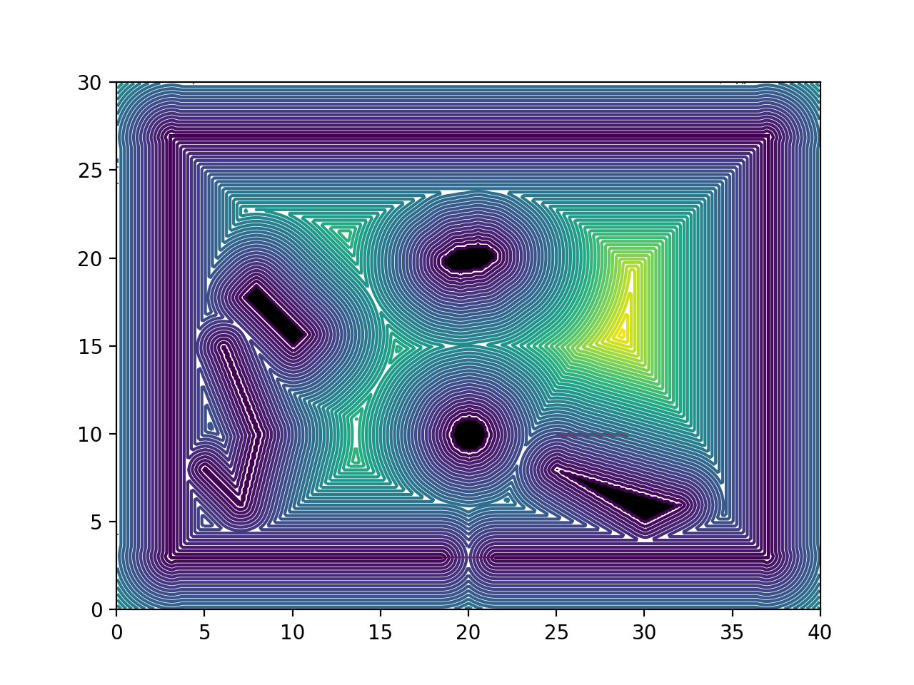
a 2D array of the size of the image representing the distance to the nearest wall (black color). This means that each pixel in the image has its distance to the nearest wall.
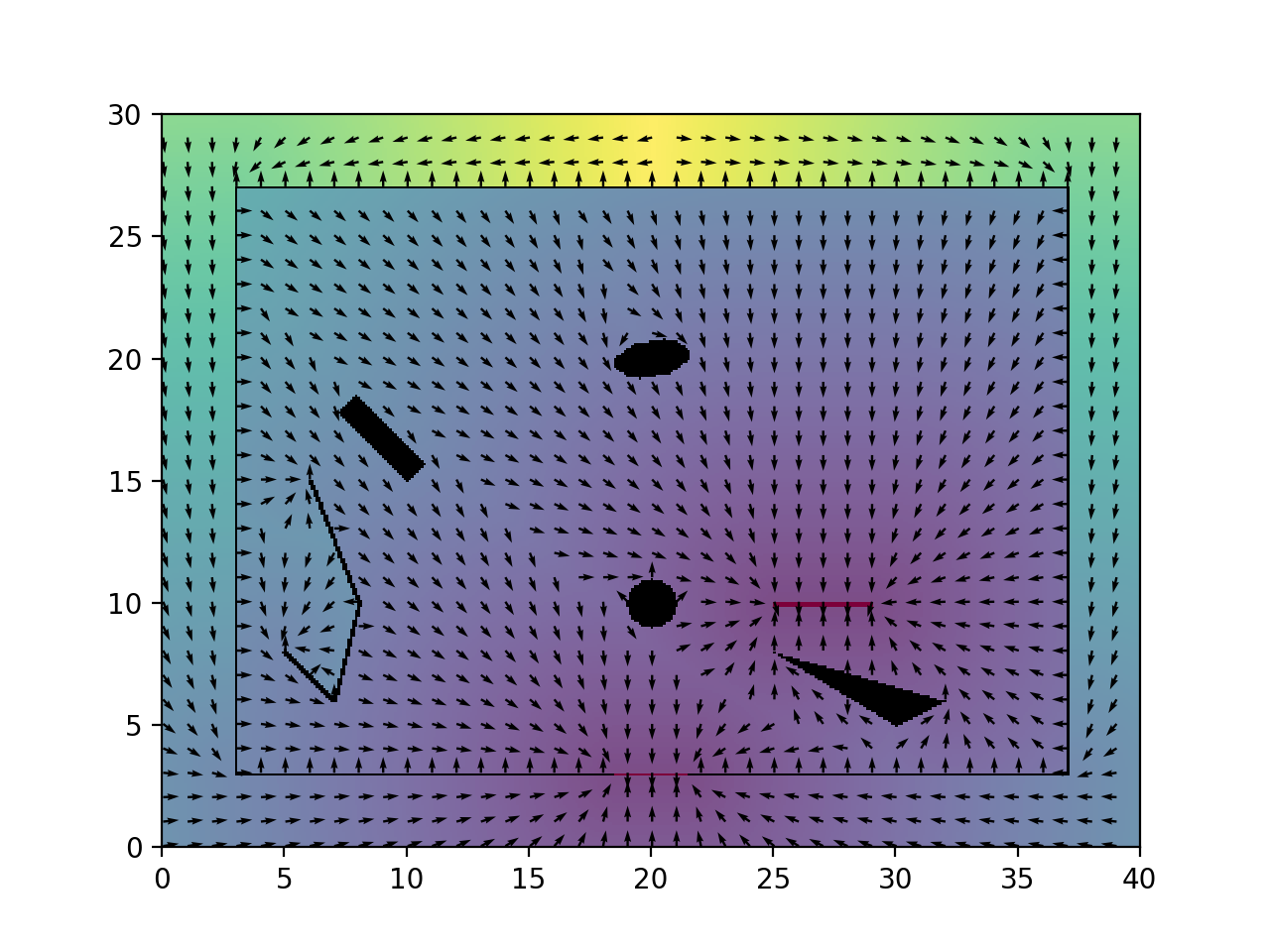
a 2D array of the size of the image representing the distance to the nearest exit (red color). The opposite of the gradient of this distance represents the desired direction for an individual desiring to reach this outcome. This desired direction is also stored in an array.
Reference : [MF2018] Chapter 8.
Manually
An example can be found in the directory
cromosim/examples/domain/
and can be launched with
python3 domain_manually_computed.py
Manually means that, from a completely white background image, the domain will be defined and drawn using Matplotlib shapes (Line2D,…). Hence, the first lines of the script build the boundary of the room (wall in black color) and the doors (in red color):
# Authors:
#     Sylvain Faure <sylvain.faure@math.u-psud.fr>
#     Bertrand Maury <bertrand.maury@math.u-psud.fr>
#
#      cromosim/examples/domain/domain_manually_computed.py
#      python domain_manually_computed.py
#
# License: GPL

from cromosim import *
import scipy as sp
import matplotlib
import matplotlib.pyplot as plt
from matplotlib.patches import Ellipse, Circle, Rectangle, Polygon, Arrow
from matplotlib.patches import Circle
from matplotlib.lines import Line2D

## Domain without a background image
pixel_size = 0.1
dom = Domain(name = 'room_400x300', pixel_size = pixel_size, width = 400, height = 300)
print(dom)

##  (x0,y1)------------------------------(x3,y1)
##    I                                     I
##    I                                     I
##  (x0,y0)-----(x1,y0)-door-(x2,y0)-----(x3,y0)
##
##                     (xd,yd)
x0 = 5.0
x1 = 19.0
x2 = 21.0
x3 = 35.0
y0 = 5.0
y1 = 25.0
xd = 20.0
yd = 2.5

## Line2D(xdata, ydata, linewidth)
line = Line2D( [x2,x3,x3,x0,x0,x1],[y0,y0,y1,y1,y0,y0], 2)
dom.add_wall(line)

## Line2D(xdata, ydata, linewidth)
line = Line2D( [x1,x2],[y0,y0], linewidth=2)
dom.add_door(line)

dom.build_domain()
which gives the following domain:
Then, the desired velocity and the wall distance can also be computed manually and added to the domain object:
## Compute manually a mask
mask = (dom.X<x0)+(dom.X>x3)+(dom.Y<y0)+(dom.Y>y1)
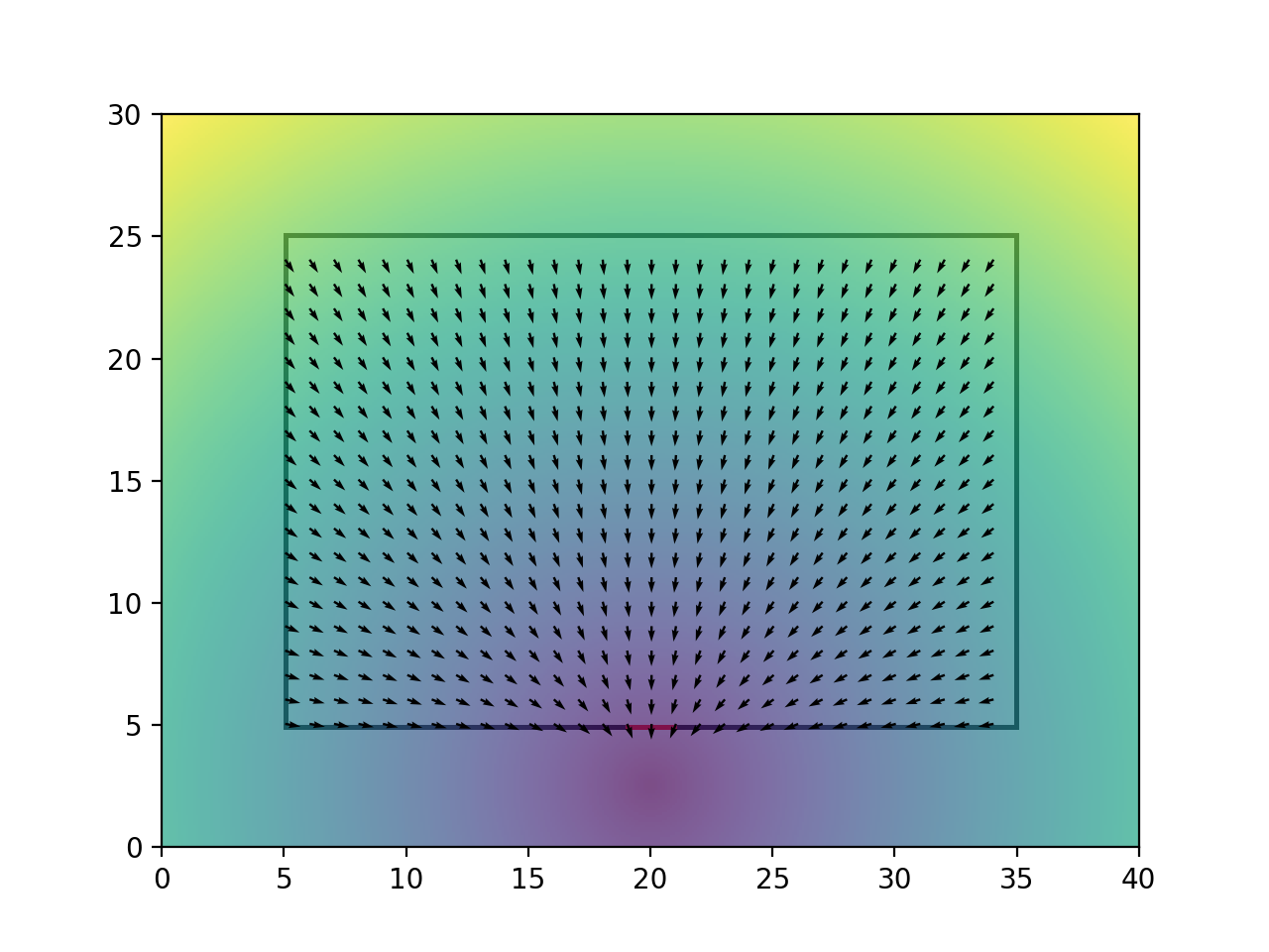
## Compute manually a desired velocity
desired_velocity_X = xd - dom.X
desired_velocity_Y = yd - dom.Y
norm = sp.sqrt( desired_velocity_X**2+desired_velocity_Y**2 )
desired_velocity_X = sp.ma.MaskedArray(desired_velocity_X/norm,mask=mask)
desired_velocity_Y = sp.ma.MaskedArray(desired_velocity_Y/norm,mask=mask)
dom.door_distance = norm
dom.desired_velocity_X = desired_velocity_X
dom.desired_velocity_Y = desired_velocity_Y
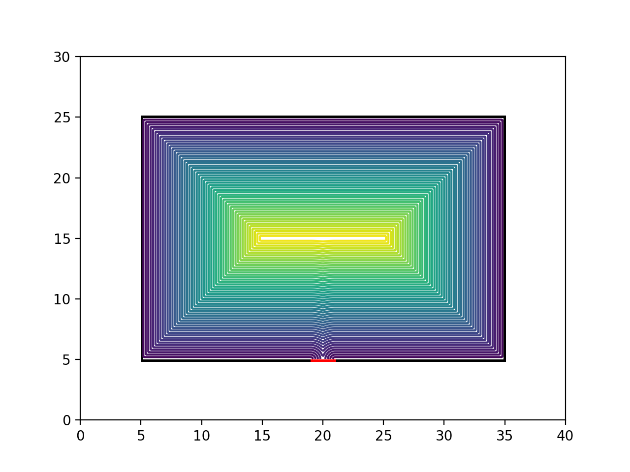
## Compute manually the wall distance
## I-------------wall2----------------I
## wall3 wall1
## I---wall0---pL--door--pR---wall0---I
dist_wall2 = y1-dom.Y
dist_wall1 = x3-dom.X
dist_wall3 = dom.X-x0
dist_wall0 = (dom.X<=x1)*(dom.Y-y0) + \
(dom.X>=x2)*(dom.Y-y0) + \
(dom.X>x1)*(dom.X<x2)*sp.minimum( \
sp.sqrt((dom.X-x1)**2+(dom.Y-y0)**2), \
sp.sqrt((dom.X-x2)**2+(dom.Y-y0)**2) \
)
wall_distance = sp.ma.MaskedArray(sp.minimum(sp.minimum(sp.minimum( \
dist_wall0,dist_wall1),dist_wall2),dist_wall3), mask=mask \
)
grad = sp.gradient(wall_distance,edge_order=2)
grad_X = grad[1]/pixel_size
grad_Y = grad[0]/pixel_size
norm = sp.sqrt(grad_X**2+grad_Y**2)
wall_grad_X = grad_X/norm
wall_grad_Y = grad_Y/norm
dom.wall_distance = wall_distance
dom.wall_grad_X = wall_grad_X
dom.wall_grad_Y = wall_grad_Y
dom.plot()
dom.plot_wall_dist(id=2)
dom.plot_desired_velocity(id=3)
## Custom plot function
fig = plt.figure(10)
ax1 = fig.add_subplot(111)
ax1.imshow(dom.image,interpolation='nearest',
extent=[dom.xmin,dom.xmax,dom.ymin,dom.ymax],
origin='lower')
ax1.contour(dom.X, dom.Y, dom.wall_distance, 50, alpha=1.0)
#ax1.imshow(wall_distance,interpolation='nearest',
# extent=[dom.xmin,dom.xmax,dom.ymin,dom.ymax],
# alpha=0.7, origin='lower')
#step = 10
#ax1.quiver(dom.X[::step, ::step],
# dom.Y[::step, ::step],
# wall_grad_X[::step, ::step],
# wall_grad_Y[::step, ::step])
#ax1.quiver(dom.X[::step, ::step],
# dom.Y[::step, ::step],
# desired_velocity_X[::step, ::step],
# desired_velocity_Y[::step, ::step])
plt.draw()
plt.show()
Automatically
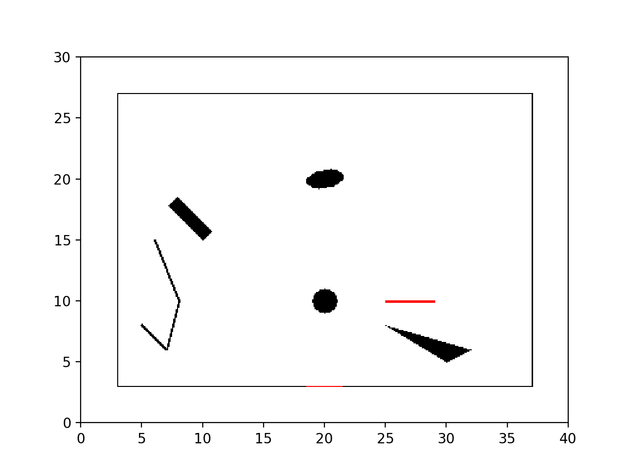
Starting from a background image drawn using three colors (red for the doors, black for the walls and white):
It is still possible to add Matplotlib shapes:
# Authors:
#     Sylvain Faure <sylvain.faure@math.u-psud.fr>
#     Bertrand Maury <bertrand.maury@math.u-psud.fr>
#
#     cromosim/examples/domain/domain_auto_computed.py
#     python domain_auto_computed.py
#
# License: GPL

from cromosim import *
import matplotlib
import matplotlib.pyplot as plt
from matplotlib.patches import Ellipse, Circle, Rectangle, Polygon, Arrow
from matplotlib.patches import Circle
from matplotlib.lines import Line2D

## Domain from a background image
dom = Domain(name = 'room_400x300', background = 'room_400x300.png', pixel_size = 0.1)

## Circle( (x_center,y_center), radius )
circle = Circle((20.0,10.0), 1.0)
dom.add_wall(circle)

## Ellipse( (x_center,y_center), width, height, angle_in_degrees_anti-clockwise )
ell = Ellipse( (20.0, 20.0), 3.0, 1.5, 10.0)
dom.add_wall(ell)

## Rectangle( (x_lower_left,y_lower_left), width, height, angle_in_degrees_anti-clockwise)
rect = Rectangle( (10.0, 15.0), 1.0, 4.0, 45)
dom.add_wall(rect)

## Polygon( xy )
poly = Polygon([[30.0, 5.0],  [32.0, 6.0],  [25.0, 8.0]])
dom.add_wall(poly)

## Line2D(xdata, ydata, linewidth)
line = Line2D( [6.0,8.0,7.0,5.0],[15.0,10.0,6.0,8.0], 2)
dom.add_wall(line)

## Line2D(xdata, ydata, linewidth)
line = Line2D( [25.0,29.0],[10.0,10.0], linewidth=2)
dom.add_door(line)
dom.build_domain()
dom.compute_wall_distance()
and then compute automatically the desired velocity and the wall distance thanks to a fast-marching method.
dom.compute_desired_velocity()
print(dom)

## Plot functions include in vap.py
dom.plot()
dom.plot_wall_dist(id=2)
dom.plot_desired_velocity(id=3)

## Custom plot function
fig = plt.figure(10)
ax1 = fig.add_subplot(111)
ax1.imshow(dom.image,interpolation='nearest',
           extent=[dom.xmin,dom.xmax,dom.ymin,dom.ymax],
           origin='lower')
ax1.contour(dom.X, dom.Y, dom.wall_distance,50,alpha=1.0)
#ax1.imshow(dom.wall_distance,interpolation='nearest',
#           extent=[dom.xmin,dom.xmax,dom.ymin,dom.ymax],
#           alpha=0.7, origin='lower')
#step = 10
#ax1.quiver(dom.X[::step, ::step],dom.Y[::step, ::step],
#           dom.wall_grad_X[::step, ::step],
#           dom.wall_grad_Y[::step, ::step])
plt.draw()

plt.show()